Convolutional Neural Networks : The Theory
Convolutional Neural Networks are the most popular Deep Learning solution for image processing. But how do they work? Read on for a mathematics and jargon free explanation!
Introduction
Convolutional Neural Networks (CNNs) are a class of Deep Artificial Neural Network that are commonly applied to image processing tasks such as object detection and identification.
If you are just getting started with Deep Learning and Artificial Neural Networks (ANNs) then I strongly recommend that you first read my Introduction to Deep Learning as this contains useful background information about Deep Learning and Artificial Neural Networks.
If you are looking for a practical example of Convolutional Neural Networks then be sure to check out Convolutional Neural Networks : An Implementation.
Convolutional Neural Networks
Basic Attributes
CNNs have a lot in common with other types of Artificial Neural Networks, including:
- Feed Forward: Feed Forward ANNs organise their nodes (or neurons) into layers, with output from each layer being fed onwards to the next layer for further processing. The majority of CNN architectures follow this convention.
- Learning via back-propagation: Whilst training, the ANN uses a Loss Function to calculate the error margin between actual output and desired output. This error margin is then used to update the ANNs weights through a process known as back-propagation, with the goal of reducing the Loss Function and therefore the error margin.
CNNs Maintain Spatial Integrity of Input Images
The below GIF shows a greyscale image of a boot from the Fashion MNIST Dataset. The purple grid shows the boundaries of the individual pixels, while the purple numbers show the value for each pixel. The image is comprised of 28x28 pixels and the value of each pixel is on a scale between 0 (lightest) and 1 (darkest).
Images as grids of pixel values is how Artifical Neural Networks, which at heart are basically mathematical engines, "percieves" images.
Some classes of Artifical Neural Networks are only be able to work with images if they are first converted to a 1D list of pixel values. The problem here is the potential loss of spatial integrity - or how pixels combine with one another to create features such as a line or shadow.
Convolutional Neural Networks maintain spatial integrity of input images. The above image would be supplied to a CNN as a 2D grid of 28x28x1.
Colour images are supplied to a CNN in the same manner, but we then need to represent the red, green and blue channels for each pixel. If our colour image is 28x28 pixels the resulting input shape would be 3D (28x28x3).
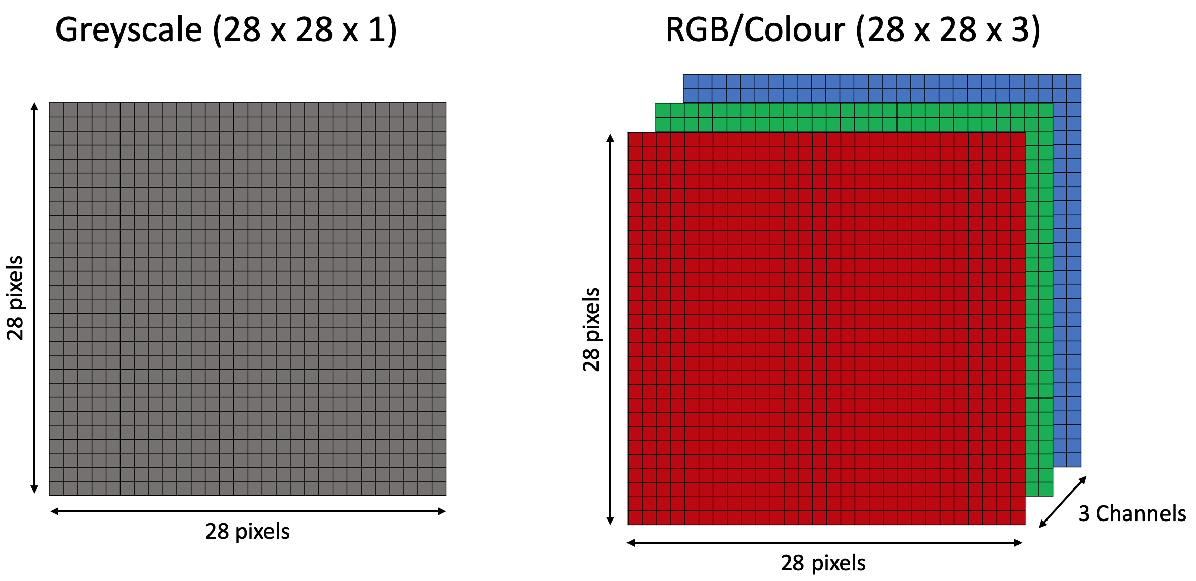
Convolutional Neural Networks process each channel individually, but keep them grouped together as the same input.
CNNs Extract Features Through Convolutional Filters
In the previous section we saw how CNNs preserve spatial integrity in incoming images. The next step is to extract features from these images through the application of convolutional filters.
In practice, convolutional filters are a set of weights that are applied to pixel values in our input image. These weights are learned and refined by a back-propagation during the training phase.
The filtering process consists of sliding a convolutional filter over an image and generating a filtered version of the image, or feature map. Convolutional filters can both accentuate and dampen specific features in input images such as curves, edges or colours. Different convolutional filters extract different features and it is the combination of the resulting feature maps that powers the CNNs predictions.
The generation of feature maps is illustrated in the following GIF:
Creating a feature map through application of a convolutional filter
The above GIF shows a 3x3 convolutional filter being applied to a 6x6 greyscale (i.e. single channel) image containing a "T" shape. Pixel values in our original image are either 0 or 1. The result of the filtering is a feature map. Here is the convolutional filter from the above GIF:
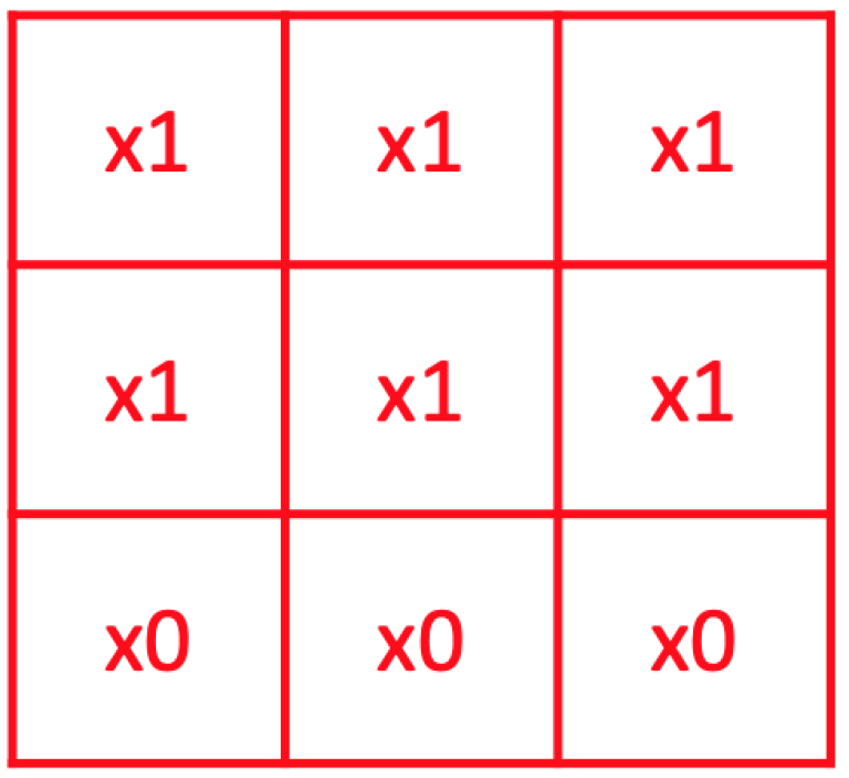
This example has been somewhat simplified to make it easier to follow. In reality pixel values are rarely binary and convolutional filters can have both positive and negative weights.
Here is an example of a set of real feature maps generated by a CNN for a given input image.
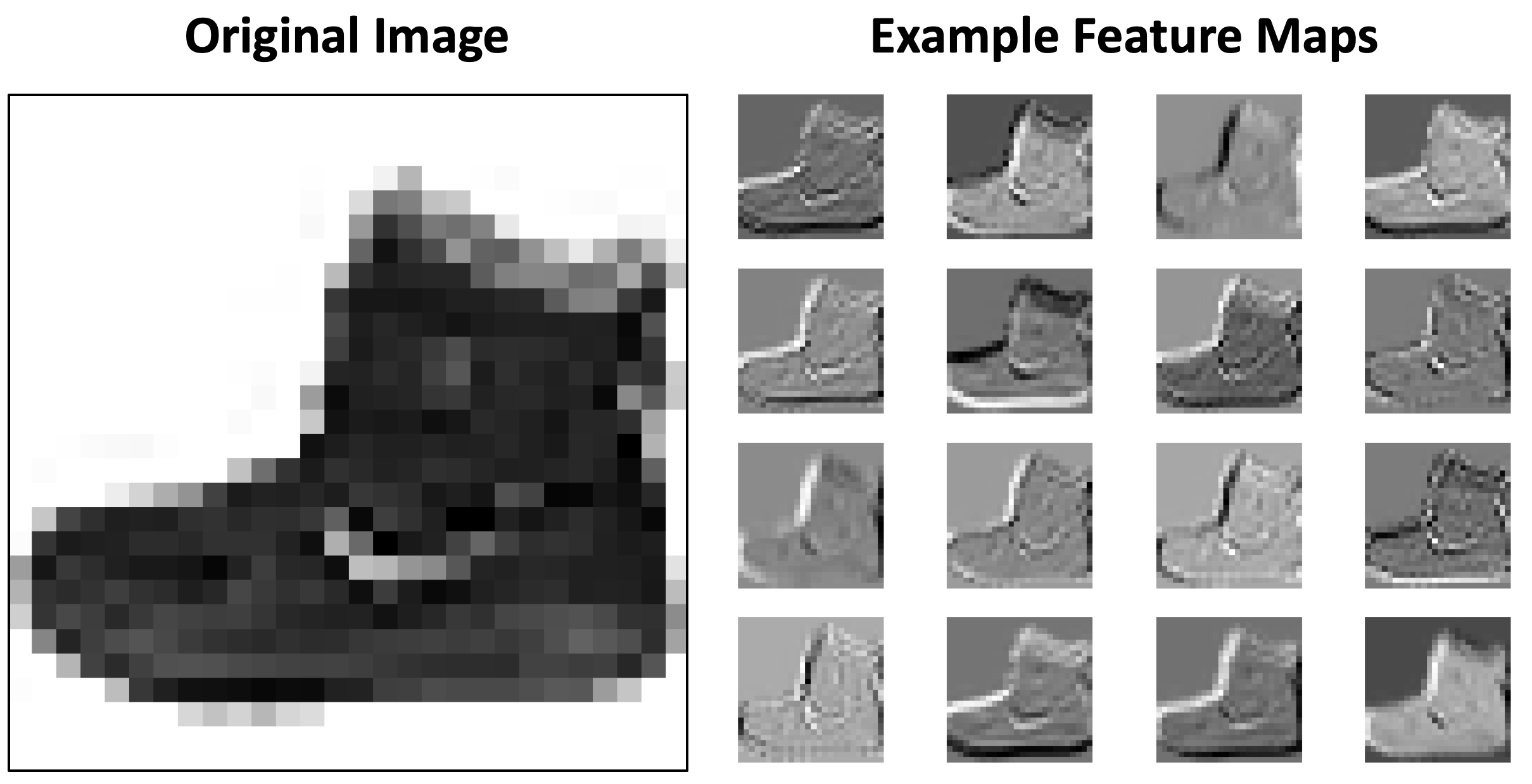
Each of the above feature maps has been generated by a specific convolutional filter. We see that different filters amplify and dampen different attributes, based on their learned biases.
When training a CNN we have various options for controlling filters, including:
- How many convolutional filters will be learned: CNNs can have tens or even hundreds of filters. Each convolutional filter generates its own feature map that is sent onwards for further processing in the CNN.
- Filter size: Convolutional filters should be large enough to take into account features spanning multiple pixels but small enough to be able to be reusable across an image. In the "T" example above the filter size is set to is 3x3 pixels.
- Stride: How many pixels does the convolutional filter move each time it process a group of pixels? In the "T" example above the stride is set to 1. Longer strides will result in smaller feature maps but can potentially miss important features.
- Padding: Should the input image be padded with empty pixels to ensure that the resulting feature map retains the same dimensions as the original input image? We are not using padding in the "T" example.
The use of convolutional filters in CNNs is inspired by the work of Hubel and Wiesel, two neuroscientists who researched how images triggered neuronal activation in the visual cortex. They suggested that visual processing is a hierarchical process which starts with the identifying of basic features which are then combined into more complex constructs.
In a similar manner, filters in CNNs allow the Neural Network to identify basic features and highlight these in specific feature maps. The feature maps can then be sent onwards in the CNN for further processing - but first they must be processed by an Activation Function.
Feature Map Enhancement via The ReLU Activation Function
Activation Functions decide on whether (and to what extent) a given node in the network sends a signal to subsequent layers. This is done by combining the node's weighted inputs and seeing if the total exceeds a given threshold.
The Rectified Linear Unit (ReLU) Activation Function is commonly used within Convolutional Neural Networks to further process feature maps before they are sent further. ReLU introduces non-linearity into our model as follows:
if node_output > 0 then
    return node_output
else
    return 0
endif
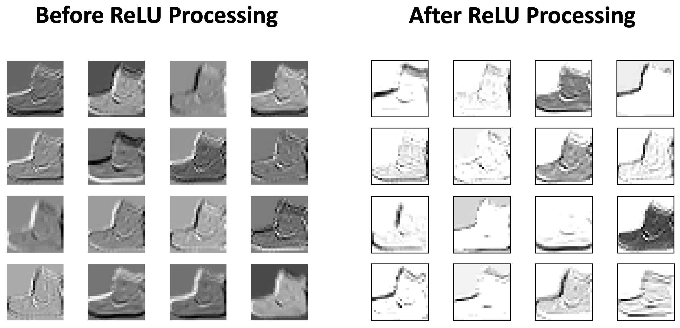
In other words, ReLU ensures that only nodes with a positive activation will send their values onwards in the CNN. Potential effects include:
- With less activated nodes there is less processing for the CNN to do.
- The nodes that are positively activated are likely working with meaningful aspects. Focusing on these can lead to better models with higher accuracy scores.
- There is less noise within the network, reducing the dangers of overfitting or learning incorrect correlations between input and desired output.
The following diagram visualises how application of the ReLU Activation Function affects the feature maps:
Dimensionality Reduction via Pooling
Another common attribute in Convolutional Neural Networks is that of Pooling. Pooling normally takes place after feature maps have been passed through the ReLU Activation Function. The goal of Pooling is to reduce the feature map size without loss of information. This in turn reduces the amount of processing required further in the CNN, saving time and resources in the training stage.
Pooling consists of passing a filter over the feature maps as follows:
As the above GIF shows, CNN pooling comes in different flavours. Three common varients are:
- Max Pooling: Takes the maximum pixel value within the filter.
- Average Pooling: Takes the average pixel value within the filter.
- Sum Pooling: Sums the pixel values within the filter.
Max Pooling is often reported to be efficient at maintaining features such as edges, and is generally seen as being a good choice to start when starting with CNNs.
In addition to choosing different Pooling filters, one can also specify the stride and the filter size. In the above example the stride is set to 2 pixels and the filter size is 2x2 pixels. A higher stride or larger filter size may result in a loss of information, so the skill is to find a good balance between efficiency and accuracy.
Here is an example of a feature map before and after Max Pooling:
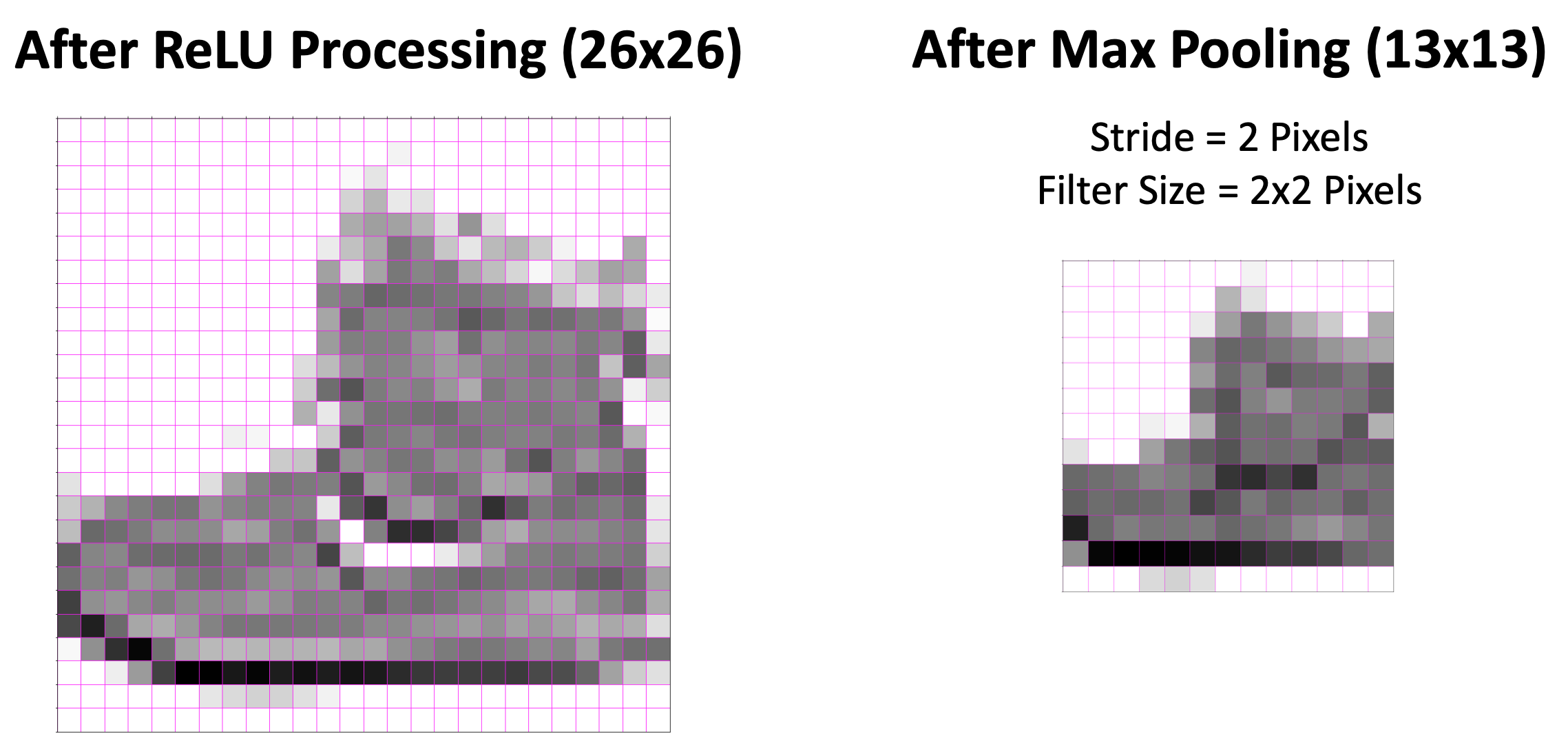
Here we see that the Max Pooling step has reduced our feature map to half of it's orignal size. This means half the processing to be done later on in the CNN.
Summary
In this article we have focused on describing the following attributes that define Convolutional Neural Networks:
- Maintain Spatial Integrity of Input Images: Images are fed into a CNN as grid of pixel values - this ensures that features spanning multiple pixels are maintained. Input can be 2D or 3D dependant upon the number of channels (for example Greyscale or RGB).
- Feature Extraction Through Convolutional Filters: The filtering process consists of sliding a convolutional filter over an image and producing a feature map. Filters both accentuate or dampen specific features in our input images such as curves, edges or colours. Different convolutional filters may extract different features from the same image and are learned during the training phase via back-propagation.
- Feature Map Enhancement via ReLU: The ReLU Activation Function is commonly used within Convolutional Neural Networks to reduce noise and enhance relevant features by replacing all negative activation values in each feature map with 0.
- Dimensionality Reduction via Pooling: The goal of Pooling is to reduce the feature maps size without loss of information. This in turn reduces the amount of processing required further in the CNN, saving time and resources in the training stage.
I hope that you enjoyed this article! Please do check out Convolutional Neural Networks : An Implementation where I use all of the above theory to create a Convolutional Neural Network using Tensorflow and Keras.
Thanks for reading!!
Mark West leads the Data Science team at Bouvet Oslo.
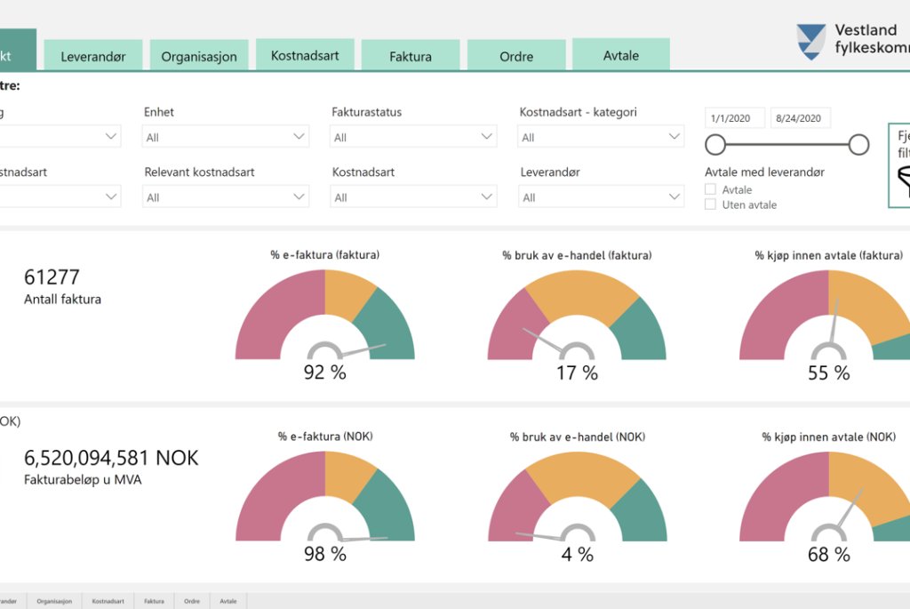
Vestland fylkeskommune
Utvikling av Power BI-rapport for innkjøpsseksjonen i Vestland fylkeskommune

Bybanen
Smart prediksjon av isdannelse gir tryggere drift av Bybanen i Bergen

Elvia
Bildeanalyse og maskinlæring for mer effektive arbeidsprosesser
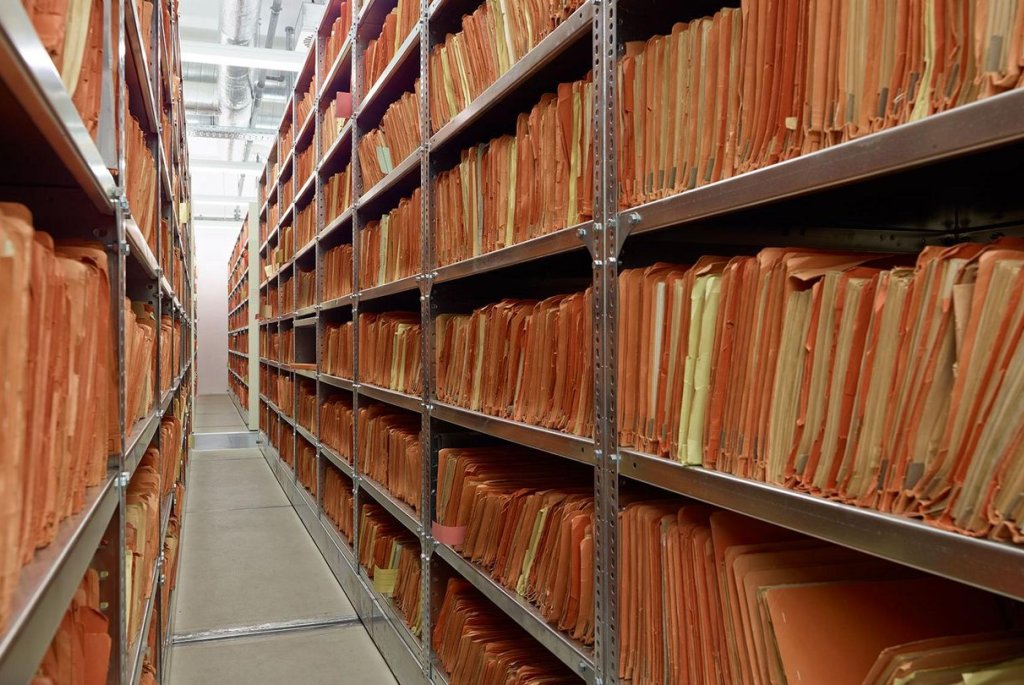
Arkivverket
Kunstig intelligens for ekstrahering av metadata fra dokumenter
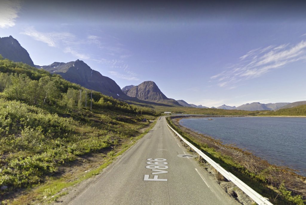
Statens Vegvesen
Takting: Smart flåtestyring gjennom flaskehalser i veinettet
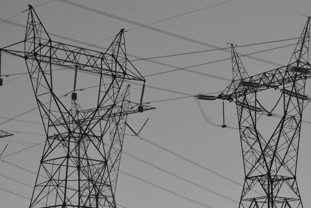
Agder Energi Nett