Convolutional Neural Networks : An Implementation
In this article I show how to implement a simple Convolutional Neural Network for image classification using TensorFlow and Keras. A link to the source code is included!

Introduction
In my previous article about the theories behind Convolutional Neural Networks I identified the following key attributes of Convolutional Neural Networks:
- Maintain Spatial Integrity of Input Images: Images are fed into a CNN as grid of pixel values - this ensures that features spanning multiple pixels are maintained. Input can be 2D or 3D dependant upon the number of channels (for example Greyscale or RGB).
- Feature Extraction Through Convolutional Filters: Convolutional filters produce feature maps that accentuate or dampen specific features in our input images.
- Feature Map Enhancement via ReLU: Reduces "noise" in feature maps and further enhances relevant features by replacing all negative activation values in each feature map with 0.
- Dimensionality Reduction via Pooling: Reduces processing requirements by reducing the size of feature maps - hopefully without loss of information.
So how do we actually build a Convolutional Neural Network? In this article I will build a CNN using the following tools:
- TensorFlow is Google's free and open source library for machine learning.
- Keras is a seperate library built on top of TensorFlow which provides a simplified API for building Artificial Neural Networks.
- Google Colaboratory is a free, cloud based Jupyter notebook environment that allows you to build and train Neural Networks from your browser.
If you are just getting started with Deep Learning and Artificial Neural Networks (ANNs) then I strongly recommend that you read my Introduction to Deep Learning as this contains useful background information about Deep Learning and Artificial Neural Networks.
Use Case : The Fashion MNIST Dataset
Before we delve into the architecture of our Convolutional Neural Network (CNN), lets first look at the dataset that we'll be working with!
The Fashion MNIST Dataset was created by Zalando and consists of a training set of 60,000 images and a test set of 10,000 images. Each image is a centered 28x28 pixel image of an item of clothing and is assigned to one of 10 classes.
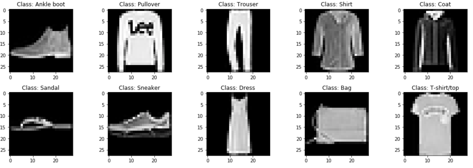
All images in Fashion MNIST are greyscale. Each pixel is represented by a single value (between 0 and 255) reflecting the darkness of that pixel.
Fashion MNIST is a well understood and simple dataset that provides good results with many ANN Architectures. It is used here so that we can focus on the CNN Architecture rather than getting bogged down in the preprocessing our chosen dataset. Another reason for choosing this dataset is that training ANNs on Fashion MNIST takes relatively short time, allowing for quick and easy experimentation.
Shut up and show me The Code!
The code for this CNN implementation (along with some examples of feature map visualisation) is available from GitHub, but I strongly recommend that you open and execute this code in Google Colaboratory (and use the GPU Runtime) in order to quickly train and test the CNN directly from your browser!
My Convolutional Neural Network
Network Overview
Convolutional Neural Networks come in many different variants, but my architecture for solving Fashion MNIST contains all of the key elements that can be found in most CNNs.
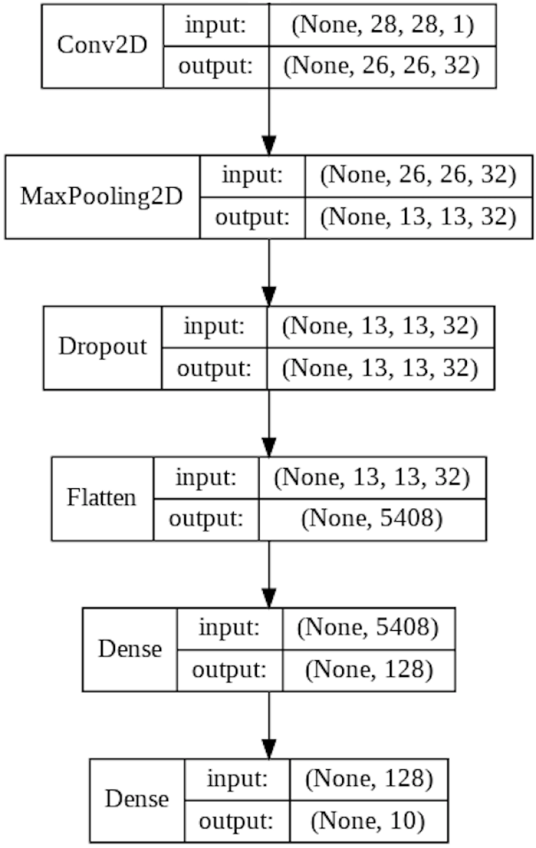
This architecture is a traditional Feed Forward Network trained via back-propagation. In the context of this image, Feed Forward means that incoming data flows downwards through the layers. During training, weights in each layer (including Convolutional Filters) are updated from the bottom up, using back-propagation.
Broadly speaking this CNN architecture performs two tasks:
- Feature Extraction: Identification of features in the input images via the application and enhacement of convolutional filters. This is primarily done in the Conv2D, MaxPooling2D and Dropout Layers.
- Classification: Mapping the identified features to a specific class. This is done in the two Dense Layers.
The bridge between these two tasks is therefore the Flatten Layer.
Confused? All will become clear as we take a closer look at each of the 6 layers.
Layer 1 : The Convolutional Layer
Convolutional Layers extract features by sliding convolutional filters over the input image and generating feature maps. This process is described further in Convolutional Neural Networks : The Theory.
The code for generating a Convolutional Layer looks like this:
# Create an empty Neural Network
model = tf.keras.models.Sequential()

# Add a Convolutional Layer to the Neural Network
model.add(
    tf.keras.layers.Conv2D(
        filters=32,
        kernel_size=(3, 3),
        strides=(1, 1),
        padding='valid',
        activation='relu',
        input_shape=(28, 28, 1)
    )
)
Key takeaways from the code:
- The Conv2D Layer will have 32 filters, each one sized as 3x3 pixels with a stride of 1. These filters will be automatically optimised during training via back-propagation.
- We are not "padding" our image with empty pixels. This will mean that the resulting feature map will be smaller than the original input image. We would use padding if we were going to have lots of Convolutional Layers and didn't want our feature maps to be scaled down too quickly.
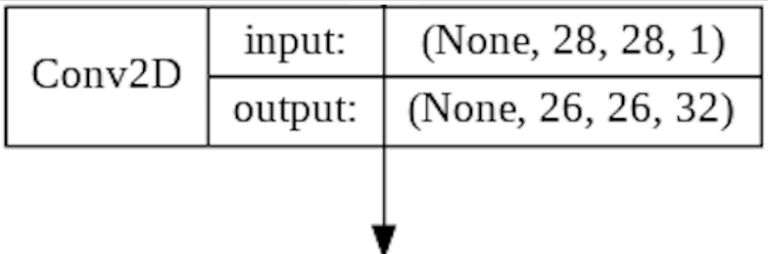
- The Conv2D Layer will generate 32 feature maps sized 26x26 pixels - for each input image. These feature maps will be further enhanced by a ReLU Activation Function before being sent on to the next layer in the CNN.
- Input to the Conv2D Layer corresponds to the shape of the images in Fashion MNIST (28x28x1).
Note that CNNs allow for multiple Convolutional Layers, allowing for subsequent Convolutional Layers to extract new features from feature maps produced by previous Convolutional Layers. This would allow for the identification of a feature hierachy in input data. In the case of Fashion MNIST this was not required due to the simplicity of the dataset.
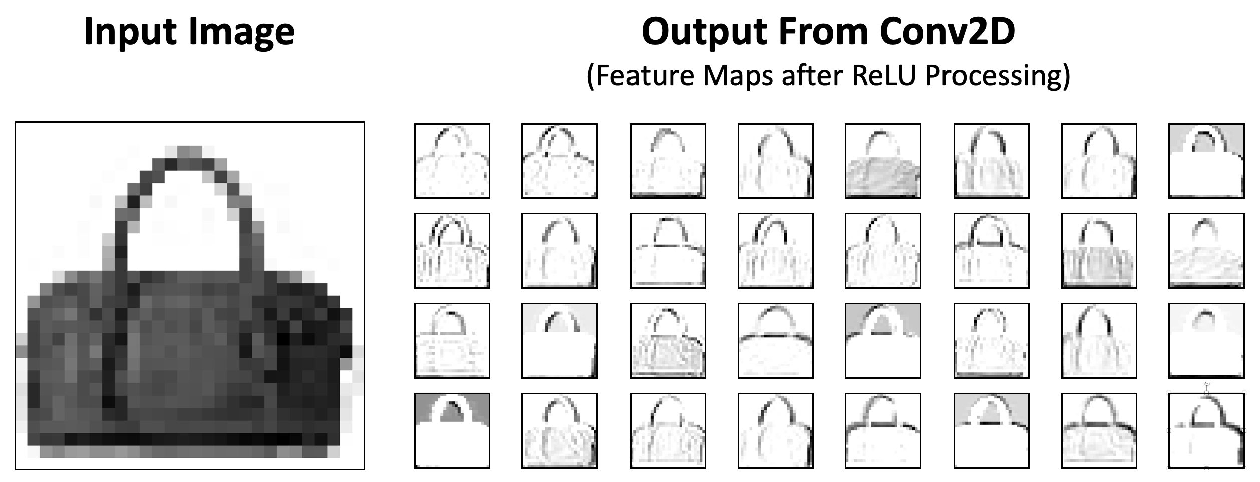
The above image shows an example of input to a trained Conv2D Layer and the resulting output. We see all 32 feature maps, each of which focus on slightly different features of the original image.
It should also be noted that feature maps are not always intuitive for humans, especially if multiple levels of Convolutional Layers have been traversed.
Layer 2 : The MaxPooling Layer
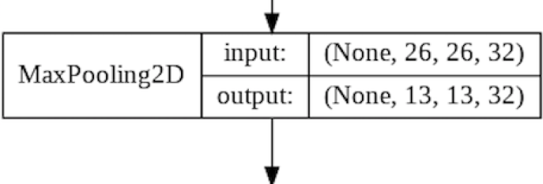
The MaxPooling Layer downsamples the feature maps, as described in Convolutional Neural Networks : The Theory. The goal here is to reduce the size of each feature map. This in turn reduces processing requirements while also scaling down the total number of parameters that the model needs to learn.
The code for generating a MaxPooling Layer looks like this:
# Add a MaxPooling Layer
model.add(
    tf.keras.layers.MaxPooling2D(
        pool_size=(2, 2),
        strides=(2, 2)
    )
)
Key takeaways from the code:
- The pool will select the maximum value from each 2x2 group of pixels.
- Setting the stride to 2 ensures that each pixel is only sampled once.
- The MaxPooling Layer has the same input shape as the Conv2D output shape. This is automatically set by Keras / TensorFlow.
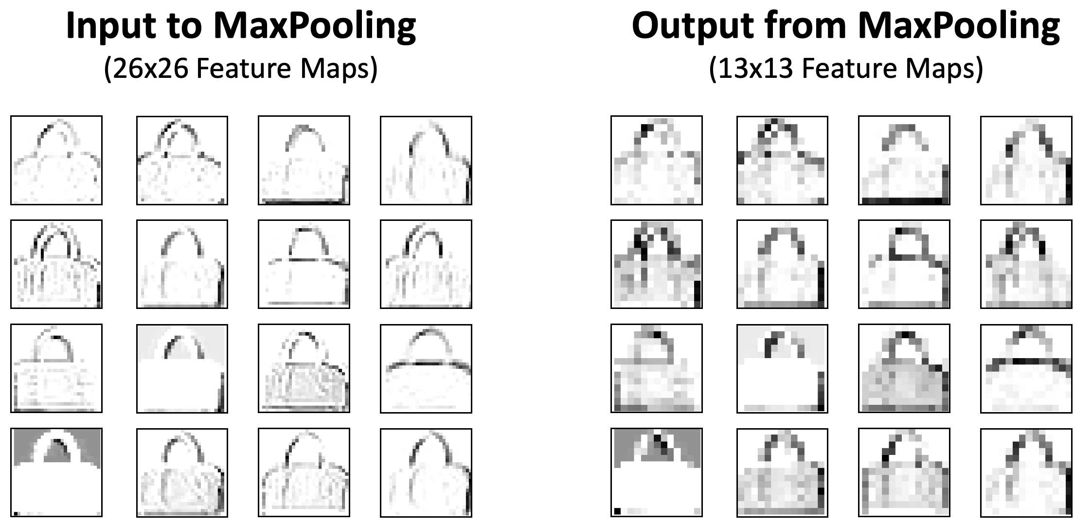
The above image shows how the MaxPooling Layer reduces our feature maps from 26x26 (676) pixels to (169) 13x13 pixels. That is a reduction of 75%!
Layer 3 : The Dropout Layer
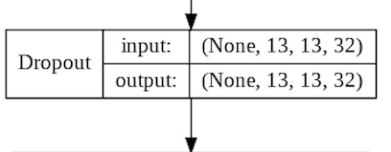
The Dropout Layer fights overfitting and forces the model to learn mulitiple representations of the same data by randomly disabling a given amount of neurons in the learning phase. The code for this is pretty simple:
model.add(
    tf.keras.layers.Dropout(
        rate=0.25
    )
)
We can see that the Dropout Layer mimics the output shape of the previous layer (this is automatically set by Keras). The only thing that happens here is that this layer will randomly disable 25% of it's nodes at a given time.
Layer 4 : The Flatten Layer
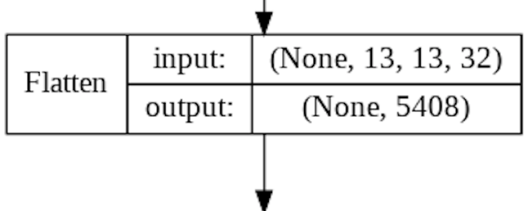
At this point we still have 32 feature maps consisting of 13x13 pixels. This is represented as a 3D array with the shape of 13x13x32. These features must be converted to a 1D list of pixel values before being sent to the Dense Layers for classification. Once again the code here is simple:
model.add(
    tf.keras.layers.Flatten()
)
The result here is simply to rearrange our 5408 nodes into a 1D list, instead of having them in a 13x13x32 array. No futher processing is done in this layer.
Layer 5 : The first Dense Layer
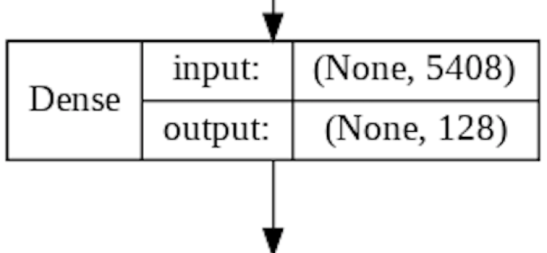
The role of the first Dense Layer is to find the correlation between our feature maps (now a 1D array of filtered values) and the desired prediction we want the CNN to make.
model.add(
    tf.keras.layers.Dense(
        units=128,
        activation='relu'
    )
)
In the above code we create a Dense Layer of 128 nodes.
As this is a Dense Layer, each of it's 128 nodes receives weighted input from all 5408 nodes in the previous Flatten Layer. These weighted inputs will be summed up and sent onwards to the same type of Activation Function (ReLU) that we used in the Conv2D Layer.
During training the weights in both Dense Layers are updated using the same mechanism (back-propagation) that updates filters in the Conv2D Layer.
Layer 6 : The second Dense Layer
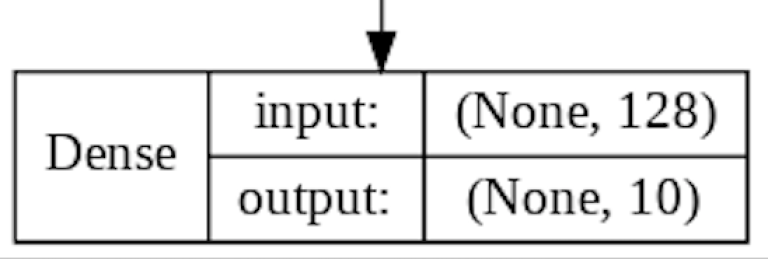
The second Dense Layer represents the final layer in our CNN. It's role is to map the 128 nodes in the previous layer to just 10 nodes that each represent a unique class in the Fashion MNIST dataset.
model.add(
    tf.keras.layers.Dense(
        units=10,
        activation='softmax')
)
As this layer is Dense, each of our 10 nodes sums up weighted inputs from all 128 nodes in the previous layer. A Softmax Activation Function then converts the summed values for each of the 10 nodes into a probability that sums to 1 across all 10 nodes. The node with the highest probability wins!
Other Model Parameters
In addition to specifying the layers of our Convolutional Neural Network, we also need to specify which loss and optimisation functions we want to use in the training of our model.
model.compile(
    loss=tf.keras.losses.sparse_categorical_crossentropy,
    optimizer=tf.keras.optimizers.Adam(),
    metrics=['accuracy']
)
Three things are being specified in this code:
- The Loss Function is used in training to calculate the deviation between the CNNs predictions and the desired output. The higher the deviation the higher the result of the Loss Function will be. Our choice of Loss Function (sparse_categorical_crossentropy) is due to our problem being a classification task where targets can only belong to a single class.
- The Optimiser Function is used in training to update weights in the Dense Layers and filters in the Conv2D Layers via back-propagation. The goal is to minimise the value of the Loss Function. We have chosen the Adam Optimiser due to its low memory requirements and current high standing in the Deep Learning world.
- Finally the metrics option tells the compiler how we want to measure and report upon our models accuracy. This does not influence how the model is trained.
For more background about back-propagation, Loss and Optimiser Functions refer to my Introduction to Deep Learning.
Summary
The code for this CNN implementation (along with some feature map visualisations) is available in Google Colaboratory for you to play around with in your browser! The code is also available in static form via GitHub.
In this article we have implemented a Convolutional Neural Network, using TensorFlow and Keras. This has given us additional insight into how CNNs process image data, and some of the possibilities that CNNs can offer.
When compared to more traditionally densely connected ANNs, CNNs are often much more efficient:
- Filters in CNNs are basically reusable weights that can be moved around images to find and match patterns no matter where they are in the image.
- In densely connected ANNs each input has its own individual weight to be calculated and updated by back-propagation.
- CNNs actively try to reduce dimensionality - for example by the application of Pooling algorithms.
- Densely connected ANNs often have redundancy and inefficiency due to each node being connected to every node in the previous and subsequent layers. This quickly leads to high processing requirements for larger images.
The use of filters also provides a couple of potential possibilities:
- Automating the feature engineering process. Feature engineering is a time consuming and often manual process where one attempts to identify the pertainent features from a given dataset. The feature extraction capabilities of CNNs can speed up and in some cases, completely automate this process.
- Transfer Learning. One can extract the Convolutional Layer (and it's filters) from a trained CNN and then reuse these in a new CNN, significantly speeding up the training of the new CNN. This of course assumes that both CNNs are working with a similar dataset.
- Visualisation of feature maps. One of the challenges with Artificial Neural Networks (ANNs) is a lack of insight in to their inner workings. As CNNs maintain the structural integrity of images in their initial layers, it is possible to visualise the feature maps and see what the CNN is prioritising. This is very useful for debugging and other insights into how the CNN is working.
In this series we have focused on using Convolutional Neural Networks for image processing, but it is important to state that the spatial awareness shown by CNNs also helps them perform well with Natural Language Processing and Time Series problems.
I do hope that you enjoyed this short series of articles about Convolutional Neural Networks! If you liked them then feel free to check out my article about Recurrent Neural Networks!
Thanks for reading!!
Mark West leads the Data Science team at Bouvet Oslo.
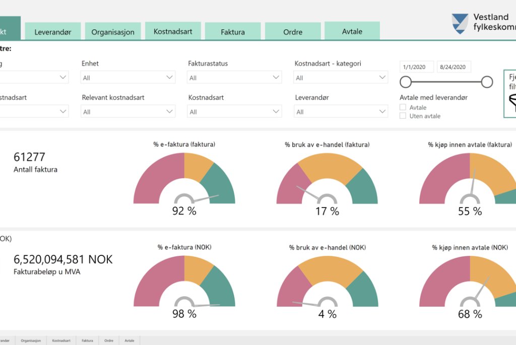
Vestland fylkeskommune
Utvikling av Power BI-rapport for innkjøpsseksjonen i Vestland fylkeskommune

Bybanen
Smart prediksjon av isdannelse gir tryggere drift av Bybanen i Bergen

Elvia
Bildeanalyse og maskinlæring for mer effektive arbeidsprosesser
Arkivverket
Kunstig intelligens for ekstrahering av metadata fra dokumenter
Statens Vegvesen
Takting: Smart flåtestyring gjennom flaskehalser i veinettet

Agder Energi Nett