Explaining Recurrent Neural Networks

Introduction

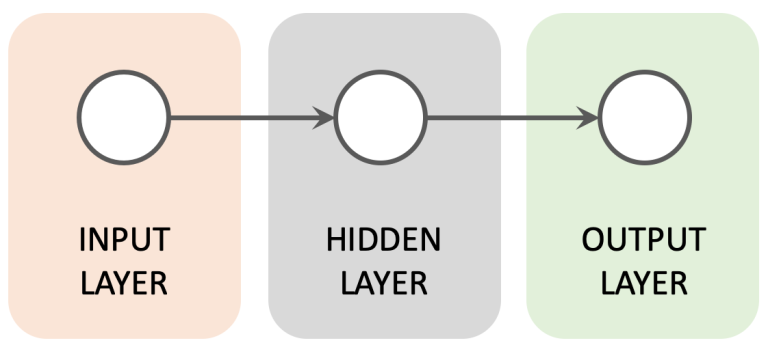
My previous articles about Deep Learning have focused upon traditional Feed Forward architectures, where incoming data travels in a single direction from the input layer to the output layer.

In this article I will introduce Recurrent Neural Networks (RNNs) which have a somewhat different architecture. RNNs have attributes that have made them very popular for tasks where data must be handled in a sequential manner, such as Natural Language Processing (NLP).

I'll start by presenting some theory about RNNs before running through an RNN implementation for sentiment analysis of IMDB movie reviews.

If you are new to Deep Learning then I would recommend that you first read my article An Introduction to Deep Learning as it gives a background for some of the concepts mentioned in this article.

Overview of Recurrent Neural Networks

Why do we need RNNs?

A potential weakness with Feed Forward architectures can be highlighted by the following animation and the question "which way is the arrow moving":

To answer this question we need to process a sequence of images while maintaining state across them. Feed Forward architectures can struggle with this type of sequential task as they do not maintain an internal state between seperate inputs that happen in a given order.

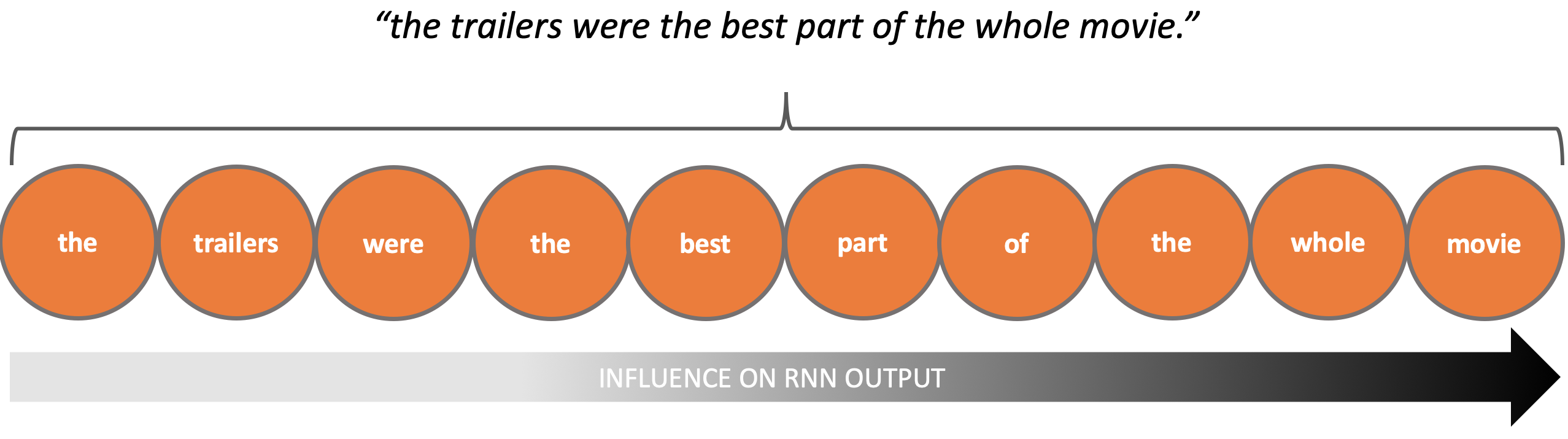
A similar issue becomes apparent when processing text:

“The trailers were the best part of the whole movie.”

To understand this sentence we again need to process the data in a given sequence - interpreting each word in the context of the words that have come before it. Once again we see that a lack of internal state could make this use case difficult to implement.

Basic attributes of RNNs

Looping through sequential data

RNNs support processing of sequential data by the addition of a loop. This loop allows the network to step through sequential input data whilst persisting the state of nodes in the Hidden Layer between steps - a sort of working memory. The following image gives a conceptual representation of how this works.

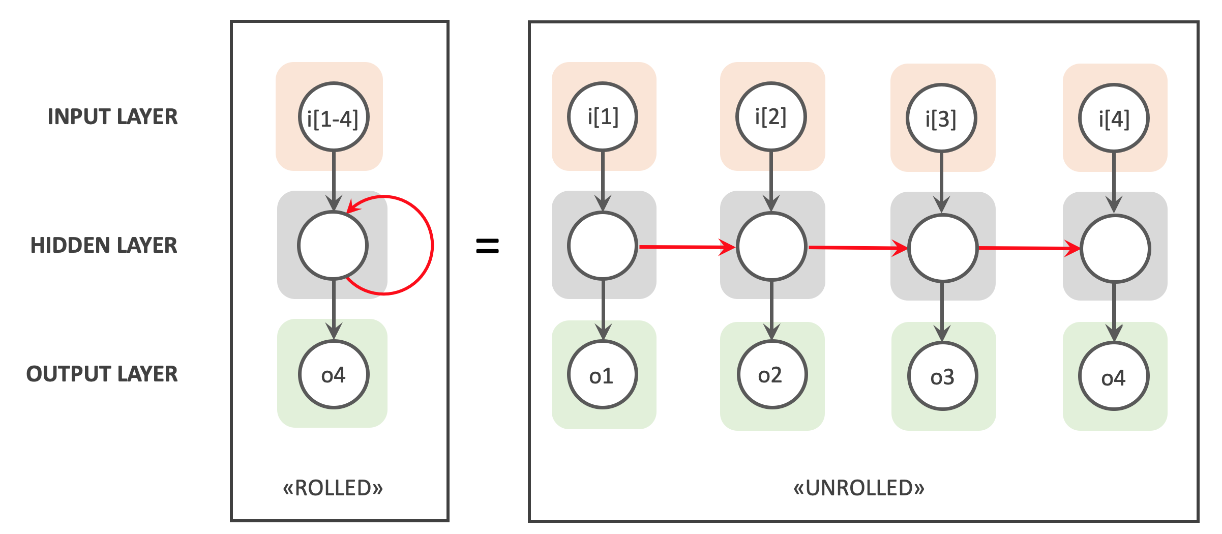
On the left hand side we see a simple RNN with input, hidden and output nodes. It takes in a sequential input with 4 elements (i[1-4]), loops through these and outputs a value of o4. In each iteration the Hidden Layer inherits the working memory from the previous iterations, as indicated by the red arrow.

On the right hand side we see an “unrolled” representation of the same RNN, which presents the RNNs loops as a chain of identical Feed Forward ANNs. These ANNs are identical, sharing the same structure, weights and activation functions. Once again the red arrows show how the working memory for each iteration is passed to the next.

The following image zooms in on the hidden node and shows how it concatenates it's current input and working memory from the previous iteration, before passing the result on to an activation function.

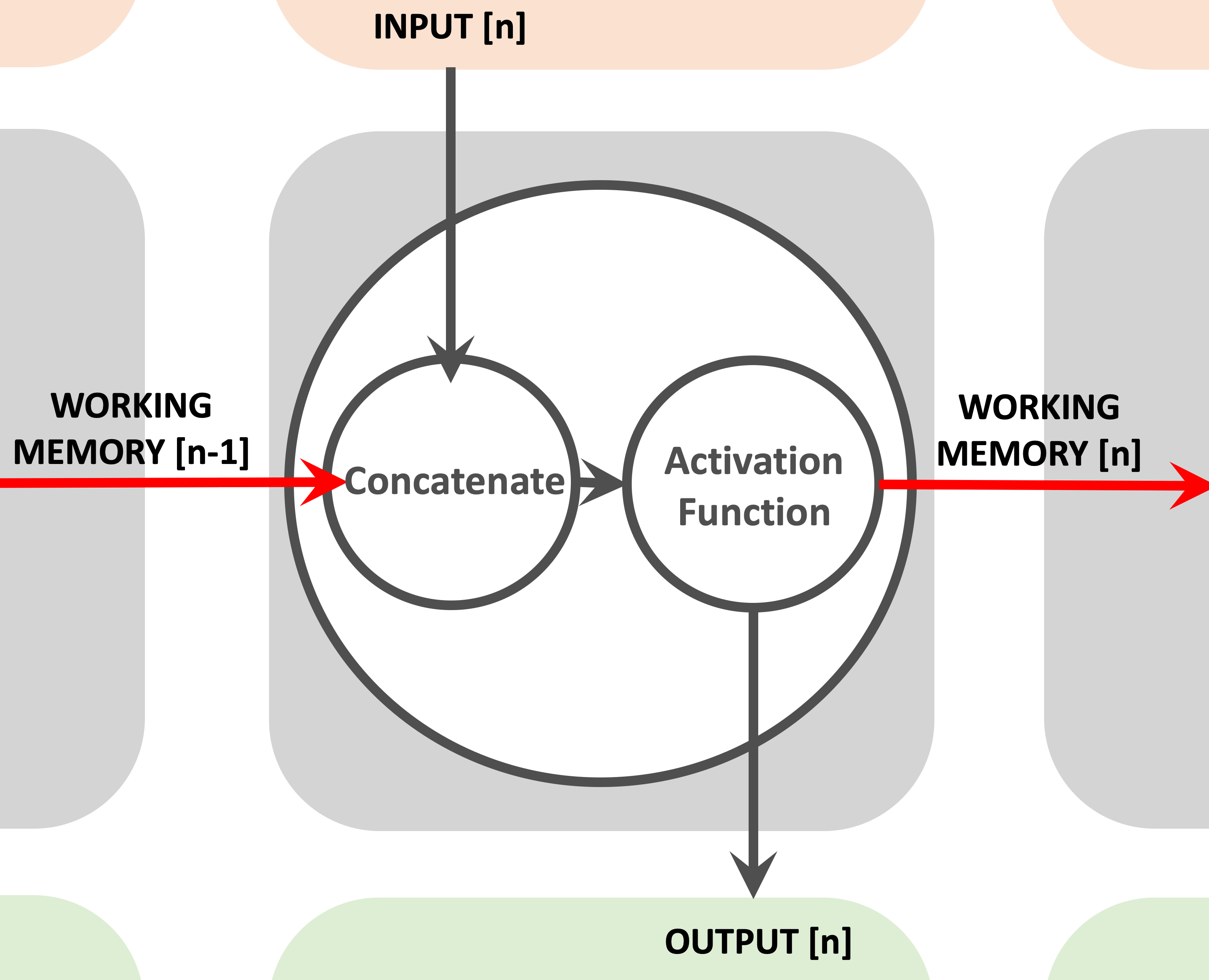
The output from the activation function is then both sent onwards to the output layer and forwarded on to the next iteration of the RNN, as the working memory of the node.

In the next section we'll see how "unrolling" an RNN is an important part of the RNN learning process.

Back-propagation Through Time

Back-propagation is the most popular technique for ANN learning. It adjusts an ANNs weights in order to reduce loss or the difference between actual and expected output, thereby optimising the ANN's performance. 

Back-propogation uses Gradient Descent to find the optimal weight values. 

Check our my Introduction to Deep Learning if you need a refresher on back-propagation and Gradient Descent.

The cyclical nature of RNNs adds an extra dimension of complexity to back-propagation. Each loop of the RNN has it's own input and output pair, while all loops share the same weights. So how and when do we update an RNN's weights?

This problem is addressed by back-propagation through time (BPTT). BPTT takes place after forward-propagation of a sequence of inputs and updates the weights of an RNN as follows:

1. The network is unrolled into a chain of ANNs. Each ANN is a copy of the original RNN, sharing the same weights and activation functions.
2. BPTT works backwards through the chain, calculating loss and error gradients across each ANN in the chain.
3. The network is rolled up and the weights are updated.

This is a greatly simplified explanation of BPTT. A deeper understanding requires a mathematical run-through which is outside the scope of this article. Note also that a lot of the back-propagation functionally is hidden by the Keras / TensorFlow API's

Limitations with RNNs

The "working memory" of standard RNNs struggles to retain longer term dependancies. The below image illustrates this problem:

This behaviour is due to the Vanishing Gradient problem, and can cause problems when early parts of the input sequence contain important contextual information.

The Vanishing Gradient problem is a well known issue with back-propagation and Gradient Descent. It can be experienced when training RNNs and also feed-forward ANNs:

• With ANNs it is the depth of the ANN that causes problems. Back-propagating over mulitple Hidden Layers results in ever diminishing error gradients, making Gradient Descent and weight optimisation difficult. 
• With RNNs it is the width of the unrolled RNN that causes problems. BPTT over multiple time steps has the same effect - ever diminishing error gradients making both Gradient Descent and weight optimisation difficult.

With both ANNs and RNNs the Vanishing Gradient problem results in a loss of information or "working memory" as one updates weights further back in the network.

Solving the Vanishing Gradient Problem with LSTM Networks

There are multiple RNN variants that aim to solve the Vanishing Gradient problem where Long Short Term Memory Networks (LSTMs) are currently the most popular. 

As with standard RNNs, LSTMs loop through sequences of data, persisting and aggregating the working memory over mutliple iterations. LSTMs also share weights and activation functions across iterations with weights being optimised via BPTT.

However LSTMs add some extra components to the mix, as the below diagram shows:

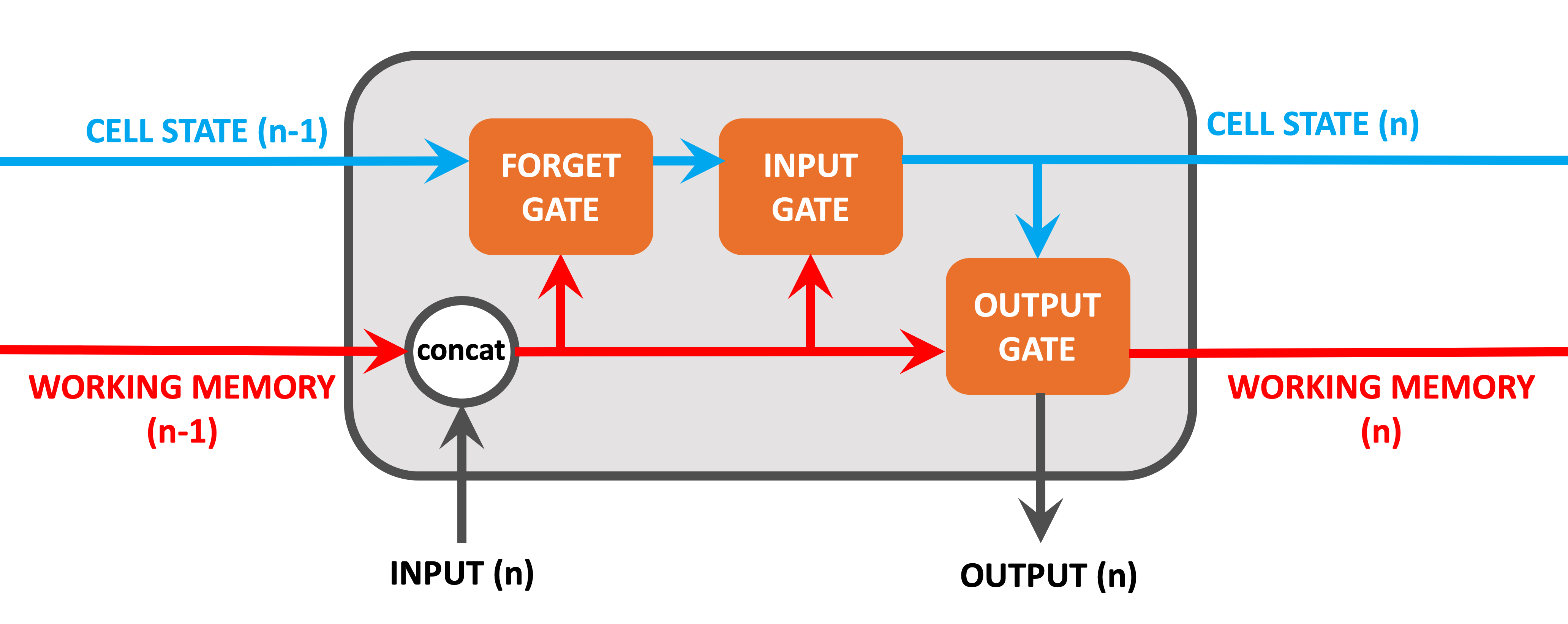
Note that the working memory as shown in this diagram acts in pretty much the same way as it would in a normal RNN.

Information coming into the node includes: 

1. Cell State from the previous iteration. This is a new component and is explained below,
2. Working memory from the previous iteration. As with traditional RNNs.
3. Input Value from the current iteration. As with traditional RNNs.

The new components on show include:

• Cell State: Cell State is the cornerstone of LSTM. It's role is to act as a long-term memory, persisting information (if required) over all iterations of the node. The Cell State can be amended to remove unecessary information or to keep important contextual information. As such it ensures that important information from early iterations will not be lost over long sequences.
• Forget Gate: The single role of the Forget Gate is to decide what information should be removed from the Cell State. This is done by performing calculations on the concatenated  working memory / Input Value and then applying these to the Cell State.
• Input Gate: The Input Gate decides what information should be added to the Cell State, based on the concatenated working memory / Input Value. 
• Output Gate: The Output Gate decides on what working memory this node will output, based on calculations on the current Cell State and the concatenated working memory / Input Value. 

Output from this node includes: 

1. Cell State (long-term memory) from this iteration.
2. Working memory from this iteration. 
3. Output Value which will be used for this iterations prediction. Note that this is the same as the working memory.

We can see that the working memory and Cell State (long term memory) interact in this type of solution. To really delve into the details of LSTM would require it's own article, so please check out Christopher Olah's definitive blog article on Understanding LSTMs if you would like more detailed information about how these work.

I think that that is enough theory for now. Lets move on with the practical part of this article!

Use Case

The IMDB Moview Review Dataset

I will be using the Keras IMDB Movie Reviews Dataset. This contains 50000 IMDB Reviews, each one classified as a "positive" or "negative" review. The data is split as follows:

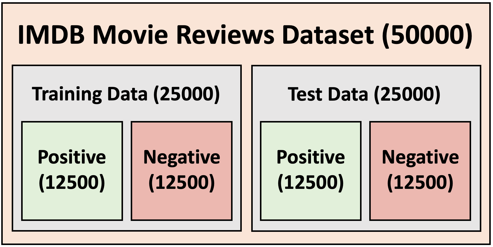
The Keras distribution of this dataset is somewhat different to the original version as it has been pre-processed:

1. Each word in the dataset is been mapped to an unique integer representing that words overall frequency in the dataset. 
2. All reviews are encoded as a sequence of the aforementioned integers, with all punctuation removed.

Having such a setup allows one to easily filter the dataset by for example only including the most common 10000 words, or even eliminating the top 20. The Keras distribution also includes a codex for mapping the numbers back to words.

Here is an example positive review directly from the dataset.

[1, 13, 296, 4, 20, 11, 6, 4435, 5, 13, 66, 447, 12, 4, 177, 9, 321, 5, 4, 114, 9, 518, 427, 642, 160, 2468, 7, 4, 20, 9, 407, 4, 228, 63, 2363, 80, 30, 626, 515, 13, 386, 12, 8, 316, 37, 1232, 4, 698, 1285, 5, 262, 8, 32, 5247, 140, 5, 67, 45, 87]

And this is how it looks once it has been translated using the codex.

<START> i watched the movie in a preview and i really loved it the cast is excellent and the plot is sometimes absolutely hilarious another highlight of the movie is definitely the music which hopefully will be released soon i recommend it to everyone who likes the british humour and especially to all musicians go and see it's great

Further Preparation of the dataset

I have made a couple of changes to the dataset:

1. Reduced the vocabulary of the entire dataset to the most popular 10000 words. This is to reduce training time, and filter out potential noise and outliers from my data.
2. Ensured that each review length is a uniform 500 words. This involves either truncating or padding reviews, depending on their original length. The goal is to ensure that all input is of a standard shape.

These changes are clearly marked in my code and you can experiment with different values to see how they affect the end result! 

Word Embedding 

Our RNN/LSTM model is going to be based on word embedding.

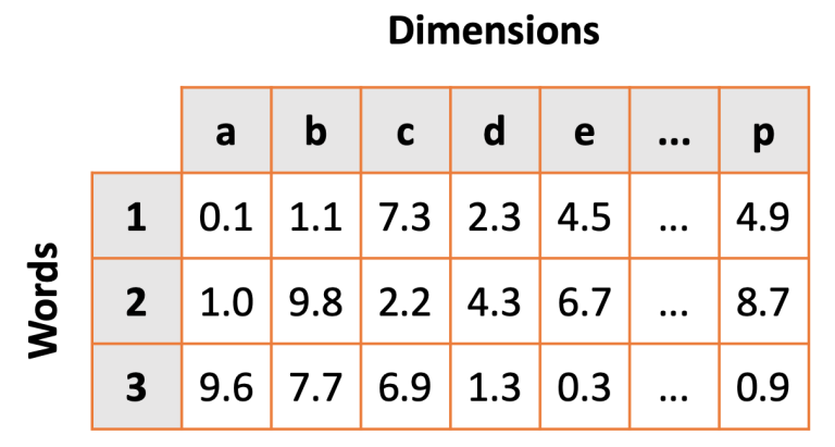
Word embedding is a popular technique for modelling word relationships by plotting them in a multi-dimensional space. The following GIF shows this concept in practice.

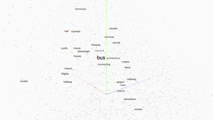
In this example a trained word embedding model has been queried for words that share the most context or meaning with the word "bus". The grey dots represent other words in the model.

Word embedding works by placing words in a multi-dimensonal space. The closer the words are, the stronger the similarity. By increasing the dimensions of our model we can capture different linguistic relationships between words. It is not unusal to encounter word embedding models with hundreds of dimensions.

One of the most exciting aspects of word embedding is that trained models have been shown to correctly interpret words that they have never seen before, by assigning the new word coordinates that match the locations of similar words in the models vocabulary.

There are many pre-trained word embedding models available. These use algorithms such as GloVe and can be inserted into your network via transfer learning. Our Deep Learning model is going to be based on word embedding. Rather than use an existing word embedding model we will create our own. 

Show me The Code!

I have used the following tools to create my LSTM:

• TensorFlow is Google's free and open source library for machine learning.
• Keras is a seperate library built on top of TensorFlow which provides a simplified API for building Artificial Neural Networks.
• Google Colaboratory is a free, cloud based Jupyter notebook environment that allows you to build and train Neural Networks from your browser.

The code for the example RNN/LSTM is available on from my GitHub, but you may want to use this link for an executable copy in Google Colab!

Note that the code is meant as a starting point, so feel free to experiement with the parameters and layers to see how your changes affects the networks performance!

Example LSTM Architecture

Overview

The goal is to create a Deep Learning Model that, after training, correctly predicts the overall sentiment (positive or negative) of IMDB movie reviews that it has never seen berfore. 

To address this I have created the following LSTM architecture.

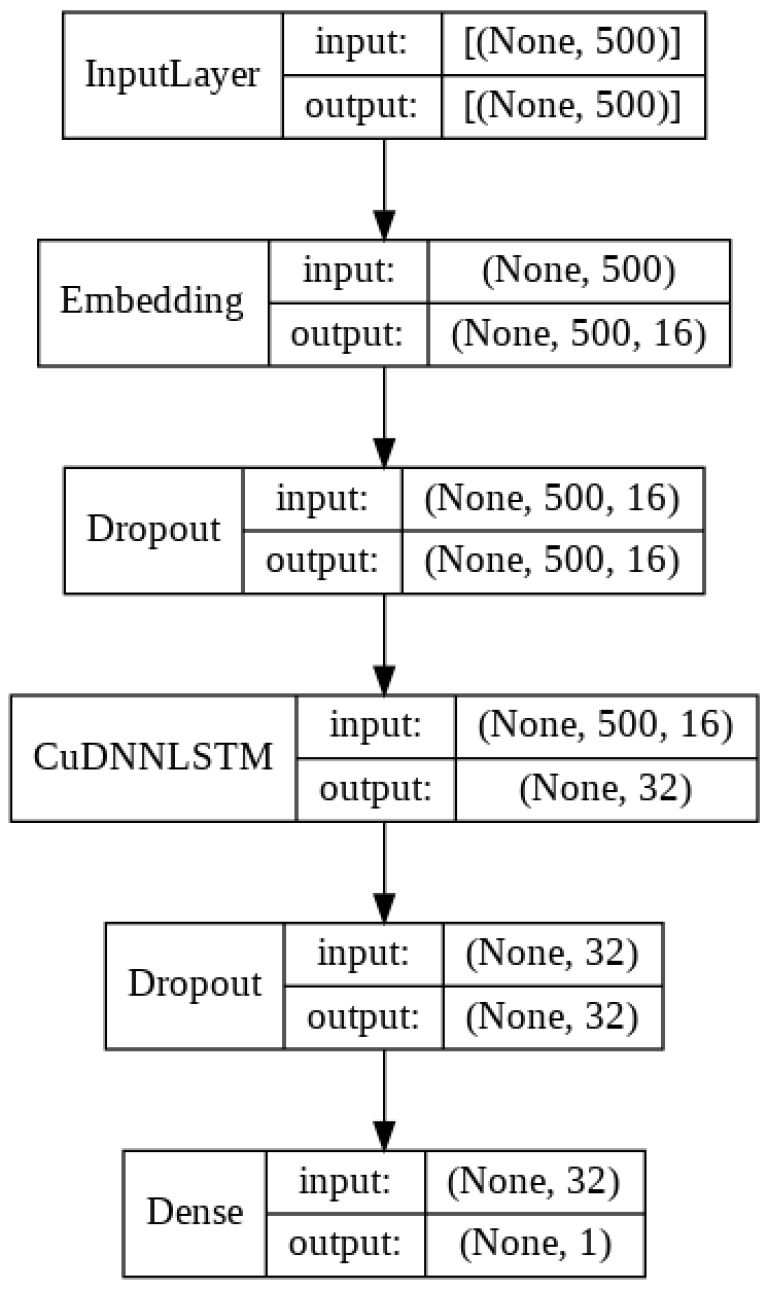
The key components here are the Embedding Layer and the CuDNNLSTM Layer:

• The Embedding Layer will learn a Word Embedding for each individual word in the the IMDB Review training set. This Word Embedding will represent each word as an integer, along with set of co-ordinates (or word vectors) that represent the meaning of that word. 
• The CuDNNLSTM Layer will learn how to differentiate between positive and negative reviews based on a sequential set of word vectors. Here the interplay between words in a sentence will be used both to guide the prediction (through forward-propagation) and also to update the Embedding Layer (through back-propagation).

Lets through the architecture in full to see what is happening with the rest of the layers.

Input Layer

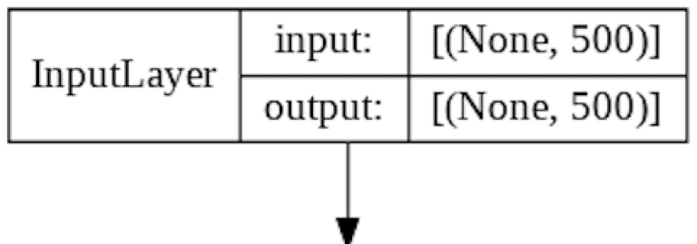
The Input Layer is automatically generated based on the input parameters of the Embedding Layer, which accepts each IMDB review as a 1D list of integer values.

Embedding Layer

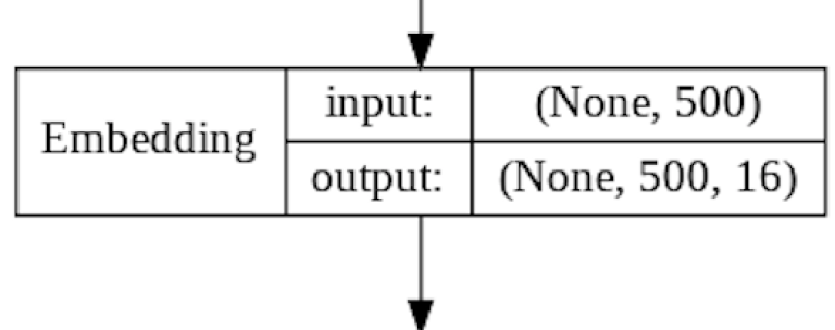
The Embedding Layer accepts a single review as a 1D list of integer values.

The Embedding Layer will learn a Word Embedding for all words in the the IMDB Review training set. Word embedding is implemented as a lookup table mapping between a given "word" and it's coordinates in the multi-dimensional word embedding space. The more dimensions you use, the “wider” the lookup table becomes. 

During training the coordinates in the lookup table are treated as weights and are updated via back-propagation during the training phase.

Here is the Keras code for implementing our Embedding Layer.

model.add(

    tf.keras.layers.Embedding(

        # The size of our vocabulary
        input_dim = 10000, 

        # Dimensions for each word
        output_dim = 16, 

        # Length of reviews
        input_length = 500 
    )
)

A quick explanation of these parameters:

1. input_dim is the amount of unique words that our entire dataset contains. In our case we have restricted our dataset to the 10000 most commonly used words.
2. output_dim is the amount of word embedding dimensions we want to map for each word.  Higher dimensional embeddings can capture fine-grained relationships between words, but require more data to learn. As our dataset is relatively small we use a small amount of dimensions.
3. input_length refers to the size of the reviews the network will process. You’ll recall that we’ve processed all our reviews so that they are 500 words long.

The output from the Embedding Layer is a 2D array containing the original review of 500 integers, plus 16 word embedding coordinates for each word.

Dropout Layer 1

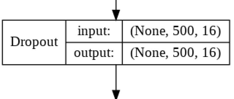
The Dropout Layer fights overfitting and forces the model to learn mulitiple representations of the same data by randomly disabling a given amount of nodes in the learning phase. The code for this is as follows:

model.add(
    tf.keras.layers.Dropout(
        rate=0.25 
    )
)

Here we will diasble 25% of the nodes that carry the output from the Embedding Layer to our LSTM Layer. Otherwise this is simply a pass through layer.

LSTM Layer

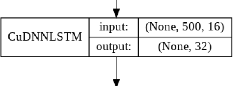
This layer learns how to differentiate between positive and negative reviews based on a sequential set of words, each represented by word vector from the Embedding Layer. 

Creating an LSTM Layer in Keras is trivial, as Keras hides the complexity (including activation functions) behind a simple API. Note that LSTM nodes commonly use both Sigmoid and Tanh Activation Functions in the different gates. For a explanation of this please check out Christopher Olah's blog article on Understanding LSTMs.

In order to speed up training I am using a Fast LSTM implementation backed by cuDNN. If you do not have a GPU available then you can use  tf.keras.layers.LSTM, but this will take a little longer.

model.add(
    tf.keras.layers.CuDNNLSTM(
        units=32
    )
)

There are few guidelines for choosing the amount of the nodes in a LSTM Layer, so my choice of 32 was guided done by trial and error. I found that 32 nodes gave good results and a very short training time.

Dropout Layer 2

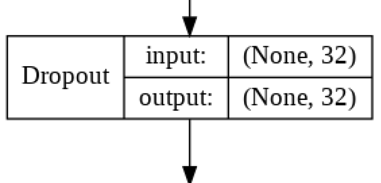
Our second dropout layer randomly disables 25% of the nodes between the LSTM Layer and the final Dense Layer, once again to fight overfitting. The code is exactly the same as the first Dropout Layer.

model.add( 
    tf.keras.layers.Dropout( 
        rate=0.25 
    ) 
)

Dense Layer

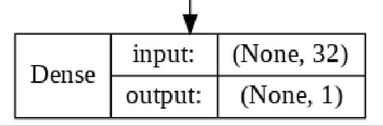
The Dense Layer represents the final layer in our LSTM. It's role is to map the 32 nodes in the LSTM Layer to a single nodes that will predict the sentiment of a given IMDB Movie Review.

model.add(
    tf.keras.layers.Dense(
        units=1,
        activation='sigmoid'
    )
)

 

Here we are using a Sigmoid Activation Function to calculate our final prediction. This is because it will give us a probability between 0 and 1. For our use case a prediction closer to 0 will indicate a negative review, while a probability closer to 1 will indicate a positive review. 

Other Model Parameters 

In addition to specifying the layers of our LSTM we also need to specify which loss and optimisation functions we want to use in the training of our model. 

model.compile(
    loss=tf.keras.losses.binary_crossentropy,
    optimizer=tf.keras.optimizers.Adam(),
    metrics=['accuracy']
)

Three things are being specified in this code: 

1. The Loss Function is used in training to calculate the deviation between the CNNs predictions and the desired output. The higher the deviation the higher the result of the Loss Function will be. Our choice of Loss Function (sparse_binary_crossentropy) is due to our problem being a binary classification task where targets can only belong one class.
2. The Optimiser Function is used in training to update weights in the Dense Layers and filters in the Conv2D Layers via back-propagation. The goal is to minimise the value of the Loss Function. We have chosen the Adam Optimiser due to its low memory requirements and current high standing in the Deep Learning world.
3. Finally the metrics option tells the compiler how we want to measure and report upon our models accuracy. This does not influence how the model is trained.

For more background about back-propagation, Loss and Optimiser Functions refer to my Introduction to Deep Learning.

Summary

The code for this LSTM implementation (along with additional code for further exploring the use case and data) is available in Google Colaboratory for you to play around with in your browser! The code is also available in static form via GitHub.

In this article we have implemented a LSTM Neural Network with the help of TensorFlow and Keras. What have we learned along the way?

1. We've learned the theory behind the RNN family of networks and seen how these can be used for handling sequential data as required by Natural Language Processing. 
2. We gained insight into how to pre-process text data for use with Neural Networks. 
3. We've learned about Word Embedding, a Natural Language Processing (NLP) technique for learning and modelling word relationships by plotting them in a multiple dimensional space. 
4. We have implemented Word Embedding and a LSTM Neural Network using TensorFlow and Keras.

It is not coincidental that we are focusing on NLP use cases in this article, as RNNs have shown most promise in this area. Other NLP use cases for RNN type networks include: 

• Predictive Text: What word comes next when typing a sentence?
• Automated Image Captioning: Instead of just generating a list of objects in a image, why not generate a short description of what the image contains? This would normally require an ANN Architecture containing both Convolutional and Recurrent Layers. 
• Machine Translation: Translation is a complex task as one needs to translate not just the individual words, but also phrases. This requires understanding of both the words and the overall sentences.

As a final note, there has been a recent interest on using Convolutional Neural Networks for some NLP tasks. Only time will tell if CNNs will take over, but it will be exciting to follow the ongoing development of Artifical Neural Networks and Deep Learning! 

I hope that you enjoyed this Introduction to Recursive Neural Networks! Feel free to check out the other articles in this series: 

• An Introduction to Deep Learning
• Convolutional Neural Networks : The Theory
• Convolutional Neural Networks : An Implementation

 

Thanks for reading!!

Mark West leads the Data Science team at Bouvet Oslo.